학습과 최적화 · Rest Math

개념에서 수식으로

먼저 이해할 내용

모델의 수식이 정해져도 계수가 자동으로 적절해지는 것은 아니다. 학습은 예측 오차를 계산하고 계수를 바꾸는 절차를 반복하는 과정이다. 이 글은 갱신 방향·이동 크기·데이터 묶음·정규화를 각각 나누어 다룬다.

기호를 먼저 읽기

θ: 학습으로 바꿀 모델 매개변수
J(θ), ℓ: 오차를 하나의 값으로 모은 목적함수
∇J: 매개변수에 대한 목적함수의 기울기
α: 갱신의 이동 크기
v, r: 이전 기울기 또는 그 제곱의 누적 정보
β: 현재 값과 이전 누적값의 비중
μ, σ²: 평균과 분산

이 글의 흐름

기본 경사하강법과 데이터 묶음의 차이를 이해한 뒤, 이동평균·모멘텀·적응형 갱신을 비교한다. 마지막에는 입력과 중간값의 정규화가 학습식에 어떻게 들어가는지 살펴본다.

주제와 표기

Training

Optimization for deep learning

모델의 예측과 학습할 계수를 분리한다

f(x;θ)는 입력 x와 계수 θ를 받아 예측값을 만든다. 학습 데이터의 정답과 예측을 비교해 J를 계산하고, θ를 바꾸어 J를 줄인다. 입력 데이터 자체와 학습으로 조정할 변수를 먼저 구별한다.

Parameterized Model

\hat{y} = f [x; θ]

input : x

parameters : θ

Training Data = {(

{\bar{x}}_{1}

y_{1}

), …, (

{\bar{x}}_{N}

y_{N}

)} = {(X,

\bar{y}

)}

Error function J = \frac{1}{2 N} \sum_{n = 1}^{N} {(y_{n} - {\hat{y}}_{n})}^{2}

{minimize}_{θ} \frac{1}{2 N} \sum_{n = 1}^{N} {(y_{n} - {\hat{y}}_{n})}^{2}

Gradient \frac{\partial J}{\partial θ}

Gradient descent

기울기의 반대로 조금 이동한다

현재 θ에서 목적함수의 기울기를 구하고 α를 곱해 뺀다. 기울기는 어느 방향이 증가 방향인지 알려주고 α는 그 방향으로 얼마나 이동할지 결정한다. α가 양수라는 조건과 현재 지점에서 미분을 평가한다는 뜻을 함께 읽는다.

Consider the objective function :

J [θ]

R^{D}

→

R

. (e . g .,

J [θ]

= 1/N∑_ (n = 1)

^{N}

f [x_{n}; θ]

y_{n}

|^2)

A first-order iterative optimization algorithm for finding a local minimum of the objective function J[θ]

Moves from the current values of parameters, $θ_{k}$ , in the opposite direction of the gradient of the objective function J[θ] w.r.t. the parameters, evaluated at $θ_{k}$

θ_{k + 1} \leftarrow θ_{k} - {α [\frac{\partial J [θ]}{\partial θ}]}_{θ = θ_{k}}

current gradient : {[\frac{\partial J [θ]}{\partial θ}]}_{θ = θ_{k}}

where α is learning rate (step size)

Taining set = {(

{\bar{x}}_{1}

y_{1}

), (

{\bar{x}}_{2}

y_{2}

), …, (

{\bar{x}}_{N}

y_{N}

)} = (X,

\bar{y}

), where

x_{n}

∈

R^{D}

and

y_{n}

∈

R

Batch = (X, \bar{y})

Mini - batch of size M = (X^{m},

{\bar{y}}^{m}

)

X^{m} = {{\bar{x}}_{m}, \dots, {\bar{x}}_{m + M - 1}}, {\bar{y}}^{m} = {y_{m}, \dots, y_{m + M - 1}}

(Full) Batch Gradient Descent ⇔ Vanilla Gradient

Resort to entire training dataset to compute the gradient of the object function

전체 데이터와 일부 데이터의 차이를 읽는다

배치 방식은 전체 데이터로 한 번의 기울기를 계산하고, 미니배치는 일부 샘플 묶음으로 갱신한다. 묶음이 하나의 샘플이면 한 샘플의 오차가 바로 갱신에 반영된다. 모델식이 달라진 것이 아니라 한 번에 기울기를 계산하는 데이터 범위가 달라진 것이다.

θ_{k + 1} \leftarrow θ_{k} - {α [\frac{\partial J [θ; X, \bar{y}]}{\partial θ}]}_{θ = θ_{k}}

The accuracy of the parameter update is high but it can be slow

Intractable for datasets that do not fit in memory

Does not allow us to update the model online (with new examples on the fly)

Mini-Batch Gradient Descent ⇔ Stochastic Gradient descent (SGD)

Consider the objective function that is the sum of errors evaluated on each batch

J [θ; X, \bar{y}] = \frac{1}{N_{M}} \sum_{m = 1}^{N_{M}} J [θ; X^{m}, {\bar{y}}^{m}]

where X^{m} and

{\bar{y}}^{m}

are training examples in mini - batch m and

N_{m}

is the number of mini batches

Mini - batch gradient descent updates parameters

θ_{k + 1} \leftarrow θ_{k} - {α [\frac{\partial J [θ; X^{k}, y^{k}]}{\partial θ}]}_{θ = θ_{k}}

Or using a batch of size 1

θ_{t + 1} \leftarrow θ_{t} - {α [\frac{\partial J [θ; {\bar{x}}_{t}, y_{t}]}{\partial θ}]}_{θ = θ_{t}}

Gradient=Steepest Descent Direction

국소 근사에서 이동 방향을 구한다

현재 값 주변에서 목적함수를 일차식으로 근사하면, 변화량의 효과는 기울기와 이동벡터의 내적으로 표현된다. 방향벡터의 길이를 정해 놓고 이 값을 작게 만드는 방향을 찾는다. 이때 목적함수를 줄이는 방향은 기울기 자체가 아니라 음의 기울기 방향이라는 앞뒤 정의를 함께 확인한다.

Let dθ = ε

\bar{v}

. Then, serach for the direction

\bar{v}

that minimizes

J [θ + d θ] \approx J [θ] + {[\nabla J [θ]]}^{T} d θ = J [θ] + {ϵ [\nabla J [θ]]}^{T} \bar{v}

under the constraint that

{| v |}^{2} = \sum_{i, j} G_{i, j} v_{i} v_{j} = {\bar{v}}^{T} G \bar{v} = 1

By the Lagrangian method, we have

\frac{\partial}{\partial \bar{v} [{ϵ [\nabla J [θ]]}^{T} \bar{v} + λ (1 - {\bar{v}}^{T} G \bar{v})]} = 0

leading to

\bar{v} = \frac{ϵ}{2 λ} G^{- 1} \nabla J [θ]

When the space isEuclidean and the coordinate system is orthogonal, then G = I, indicating that the gradient is the steepest descent direction

Convex function

볼록성은 두 점 사이의 함수값 관계이다

볼록함수 식은 두 점의 함수값을 섞은 값과 두 점을 섞은 위치의 함수값을 비교한다. 그림의 굽은 모양을 외우기보다 부등호의 어느 쪽이 큰지 읽는다. 안장점은 단순히 값이 작거나 큰 점과 다른 형태로 원문에서 구별한다.

α f [x_{1}] + (1 - α) f [x_{2}] \geq f [α x_{1} + (1 - α) x_{2}]

Concave

Saddle Points

Neural Network $f_{θ}$ [x]

반복 갱신의 방향과 크기를 따로 기록한다

θₖ에 이동방향 v와 크기 α를 곱해 더하면 다음 θ가 된다. argmin은 이 반복의 목표가 되는 매개변수를 뜻한다. 중간 유도에서 기호가 바뀌어 보이는 줄은 정의와 차원을 확인하며 읽고, 모든 줄이 별도 조건 없이 같은 식이라고 확대하지 않는다.

θ : layer sum

Sample (Training Set) : S

Training : Algorithm (S, ℓ) = θ^{*}, {f_{θ}}^{*} [x]

loss : ℓ [f_{θ} [x], y]

square loss: ℓ = \frac{1}{2 N} \sum_{n = 1}^{N} {(f_{θ} [x_{n}] - y_{n})}^{2}

{argmin}_{θ} ℓ [f_{θ} [x], y]

{argmin}_{θ} ℓ [θ]

Iterative methods

initial θ_{0} \to θ_{1} \to θ_{2} \to \dots \to θ_{k} \to θ^{*}

θ_{k} \leftarrow θ_{k - 1} + α υ_{k - 1}

step size : α

direction : υ_{k - 1}

ℓ [θ + d θ] < ℓ [θ]

d θ = ϵ υ, {| υ |}_{2} = 1

ℓ [θ + d θ] \approx ℓ [θ] + \nabla ℓ^{T} [θ] d θ (first - order approximation)

= ℓ [θ] + \nabla ℓ^{T} [θ] (ϵ υ)

{minimize}_{υ} \nabla ℓ^{T} [θ] (ϵ υ) + λ (1 - υ^{T} υ)

\frac{\partial}{\partial υ [\nabla ℓ^{T} [θ] (ϵ υ) + λ (1 - υ^{T} υ)]} = ϵ \nabla ℓ [θ] - 2 λ υ = 0

2 λ υ = ϵ \nabla ℓ [θ]

λ = \frac{ϵ}{2 λ} \nabla ℓ [θ]

Problem

하강 방향인지 내적의 부호로 확인한다

현재 기울기와 v의 내적이 음수이면 작은 이동에서 목적함수가 줄어드는 방향임을 판단할 수 있다. v를 음의 기울기로 두면 내적이 음의 노름 제곱이 된다. 다만 기울기가 0인 경우는 엄격한 감소가 보장되는 경우와 구별한다.

We consider the objective function (loss function, error function)

J [θ]

R^{D}

→

R

For instance, the square loss is given by

J [θ] = \frac{1}{2 N} \sum_{n = 1}^{N} {| f [x_{n}; θ] - y_{n} |}^{2}

Traning (or learning) involves finding a minimizer of

J [θ]

a r g min_{θ} J [θ]

General form of iteration methods

θ_{k + 1} \leftarrow θ_{k} + α_{k} v_{k}

step size :

α_{k}

direction : v_{k}

Definition

For a given point θ∈

R^{D}

, a direction v∈

R^{D}

is called a decent direction if there exists

\bar{α}

such that

J [θ + α v] < J [θ], \forall α \in (0, \bar{α})

Lemma

For a point θ∈

R^{D}

, any direction v satisfying

< \nabla J [θ], v >= \nabla J^{T} [θ] \cdot v < 0

is a descent direction

Certainly - ∇

J [θ]

is a descent direction, since

< \nabla J [θ], - \nabla J [θ] >= - {| \nabla J [θ] |}^{2} < 0

Suppose that you are sitting at a point θ∈

R^{D}

and looking at the value of the function

J [θ]

in all directions around you .

The direction with the maximum rate of decrease is along - ∇

J [θ]

Exponentially Weighted Moving Average

최근 값에 더 큰 비중을 두어 누적한다

vₜ=βvₜ₋₁+(1−β)θₜ는 이전 평균과 새 값을 섞는 식이다. 이를 반복해서 펼치면 오래된 값에는 β의 더 높은 거듭제곱이 붙는다. β=0.9에 대한 1/(1−β)=10은 대략적인 기억 길이를 설명하는 관계이며, 정확히 최근 10개만 사용하는 창 평균은 아니다.

Suppose that we are given

θ_{1}

θ_{2}

θ_{3}

, …

Moving average of

θ_{t}

is calculated as

v_{t} = β v_{t - 1} + (1 - β) θ_{t}

β \in [0, 1], β = 0.9

v_{0} = 0

v_{1} = β v_{0} + (1 - β) θ_{1} = (1 - β) θ_{1}

v_{2} = β v_{1} + (1 - β) θ_{2} = (1 - β) (β θ_{1} + θ_{2})

v_{t} = (1 - β) (β^{t - 1} θ_{1} + β^{t - 2} θ_{2} + \dots + θ_{t})

≈which approximately average over 1/(1 - β) samples

β = 0.9 \Rightarrow \frac{1}{1 - β} = 10

Bias Correction

초기값의 영향을 보정한다

누적값을 0에서 시작하면 초기에 값이 작아지는 효과가 생긴다. vₜ를 1−βᵗ로 나누는 식은 이 초기 편향을 보정하기 위한 것이다. 원문의 수치 예시에는 근삿값처럼 읽어야 하는 줄이 있으므로, 뒤의 등호를 모두 정확한 산술 등식으로 해석하지 않는다.

Use

v_{t}

/(1 -

β^{t}

) instead of

v_{t}

(useful during initial phase)

\frac{v_{1}}{1 - 0.9} = 10 v_{1}

\frac{v_{2}}{1 - {0.9}^{2}} = 5 v_{2}

\frac{v_{10}}{1 - {0.9}^{10}} = v_{10}

Gradient Descent with Momentum

모멘텀은 기울기의 누적 방향을 사용한다

매번 현재 기울기만 쓰는 대신 이전 누적 기울기와 새 기울기를 섞는다. 여러 단계에서 같은 방향이 유지되면 그 경향이 갱신에 남고, 방향이 자주 바뀌면 일부 변화가 서로 완화된다. 이후 θ 갱신은 이 누적값 v에 α를 곱해 적용한다.

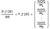
Recall gradient descent

θ_{t + 1} = θ_{t} - α [\nabla J [θ_{t}]]

where α is the step size

Gradient descent with momentum uses moving averages of gradients to update parameters

v_{t + 1} = β v_{t} + (1 - β) [\nabla J [θ_{t}]]

θ_{t + 1} = θ_{t} - α v_{t + 1}

θ = (\begin{matrix} θ_{1} \\ θ_{2} \\ : \\ θ_{D} \end{matrix})

$수식$

Alternatively, we write the gradient descent with momentum as

$수식$

When gradients keep pointing in the same direction, this will increase the size of the steps taken towards the minimum

When the gradient keeps changing direction, momentum will smooth out the variations

Manhattan-Learning Rule

기울기의 크기 대신 부호로 이동한다

Manhattan 규칙은 각 가중치의 기울기가 양수인지 음수인지에 따라 일정한 크기로 이동한다. 기울기가 크다고 이동량을 더 크게 만드는 구조가 아니다. 0인 경우의 분기도 함께 읽으면 좌표별 갱신 규칙이 명확해진다.

Acts independently on each weight

Update depend on the sign of the gradient

The update - value is constant through iterations

{θ_{i}}^{t + 1} = {θ_{i}}^{t} + Δ θ_{i}

where

θ_{i}

= {{{-

Δ_{0}

, if ∂

J

/∂

θ_{i}

>0}, {

Δ_{0}

, if ∂

J

/∂

θ_{i}

<0}, {0, else}}

where

Δ_{0}

is the update - value, which is a problem - dependent constant

Resilent Backprop (Rprop)

Rprop은 좌표별 이동 크기를 조절한다

연속한 두 기울기의 부호가 같으면 그 좌표의 이동 크기를 늘리고, 부호가 바뀌면 줄이는 구조이다. η⁺와 η⁻는 이 증가·감소의 비율을 나타낸다. 원문은 전체 배치 맥락을 설명하므로, 미니배치에 같은 특성이 그대로 보장된다고 가정하지 않는다.

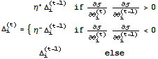
Used for full batch learning

Goal : Resolve the problem that gradients may vary widely in magnitudes

Acts independently on each weight

Extension of Manhattan learning rule

Combines the idea of using the sign of the gradient with the idea of adapting the step size individually for each weight

The update - value,

Δ_{i}

, for each weight evolves during the learning process

Increase the learning rate for a weight multiplicatively if signs of last two gradients agree

Else decrease learning rate multiplicatively

Initialize all updates at iteration 0 to constant value

The update - value,

Δ_{i}

, for each weight evolves during the learning process

$수식$

where 0<

η^{-}

<1<

η^{+}

. (typical setting :

η^{+}

= 1.2,

η^{-}

= 0.5)

Update weights :

{θ_{i}}^{t + 1}

{θ_{i}}^{t}

+ Δ

{θ_{i}}^{t}

, where

{θ_{i}}^{t}

= {{{-

{Δ_{i}}^{t}

, if ∂

J

/∂

θ_{i}

>0}, {

{Δ_{i}}^{t}

, if ∂

J

/∂

θ_{i}

<0}, {0, else}}

Does not work well for mini - batch learning

AdaGrad: Adaptive Gradient

AdaGrad는 누적 제곱으로 보폭을 나눈다

각 매개변수에 대해 지금까지의 기울기 제곱을 모으고, 그 제곱근이 갱신식의 분모에 들어간다. 누적량이 큰 좌표는 같은 현재 기울기에서도 상대적으로 작은 이동을 하게 된다. 원문의 i 좌표와 분모 첨자 표기는 대응을 확인하며 읽는다.

A different step size for every parameter

θ_{i}

at every time step t .

{θ_{i}}^{t + 1} = {θ_{i}}^{t} - \frac{α}{\sqrt{{G_{1, 1}}^{t} + ϵ}} \nabla J [{θ_{i}}^{t}]

where

{G_{i, i}}^{t}

= ∑_ (j = 1)^t (∇

J [{θ_{i}}^{j}]

)^2 contains the sum of squares of the gradients w . r . t .

θ_{i}

up to time step t

G_{i}

mi^(t) represents the diagonal entries of the matrix

G^{t}

which is calculated as

G^{t} = diag [\sum_{j = 1}^{t} (\nabla J [θ^{j}]) {(\nabla J [θ^{j}])}^{T}]

RMSProp

RMSProp은 최근 제곱기울기에 더 비중을 둔다

모든 과거 제곱을 계속 더하는 대신 지수이동평균으로 r을 갱신한다. 현재 기울기를 √(r+ε)로 나누어 좌표별 크기를 조절한 뒤 α를 곱한다. 여기서 제곱과 나눗셈은 원문에 적힌 대로 성분별 연산이다.

RMSProp = Rprop + S G D

Adaptive individual learning rate for each weight

Instead of accumulating all past squared gradients, the moving average is used to scale the step size

Update parameters

θ_{t}

r_{t + 1} = β r_{t} + (1 - β) {(\nabla J [θ_{t}])}^{2} (element - wise square)

v_{t + 1} = \nabla \frac{J [θ_{t}]}{\sqrt{r_{t + 1} + ϵ}} (element - wise division)

θ_{t + 1} = θ_{t} - α v_{t + 1}

ADAM Optimization

Adam은 방향 누적과 크기 누적을 함께 사용한다

v에는 기울기를, r에는 기울기의 제곱을 누적한다. 두 누적값에 초기 편향 보정을 적용한 뒤, 보정한 v를 보정한 r의 제곱근으로 나누어 갱신한다. 분자와 분모가 서로 다른 정보를 담는다는 점이 핵심이다. 원문에 생략된 안정화 상수를 새로 넣은 식으로 설명하지는 않는다.

Uses estimations of first and second moments of gradient to adapt the learning rate for each weight of the neural network

Adaptive individual learning rate for each weight

ADAM = momentum + bias correction + RMSProp

v_{t} = β_{1} v_{t - 1} + (1 - β_{1}) (\nabla J [θ_{t - 1}])

r_{t} = β_{2} r_{t - 1} + (1 - β_{2}) {(\nabla J [θ_{t - 1}])}^{2} (element - wise square)

{v_{t}}^{bc} = \frac{v_{t}}{1 - {β_{1}}^{t}}

{r_{t}}^{bc} = \frac{r_{t}}{1 - {β_{2}}^{t}}

θ_{t} = θ_{t - 1} - α \frac{{v_{t}}^{bc}}{\sqrt{{r_{t}}^{bc}}} (element - wise division)

Learning Rate Decay (Step Size)

학습이 진행되며 이동 크기를 줄인다

α₀는 처음 설정한 이동 크기이고, 이후 식은 epoch나 반복 횟수에 따라 α를 줄이는 예이다. 역수, 지수, 제곱근 형태가 각각 얼마나 빠르게 감소하는지 비교한다. 원문은 여러 선택안을 나열한 것이므로 하나의 필수 규칙으로 읽지 않는다.

Slowly reduce the step size α

1 epoch = 1 pass through whole training examples

Strategies (η = decay rate&Ω = epoch number)

α = \frac{1}{1 + η Ω} α_{0}

α = {0.95}^{Ω} α_{0}

α = \frac{k}{\sqrt{Ω}} α_{0}

α = \frac{k}{\sqrt{t}} α_{0}

or α is manually set such that the value of constant is decreasing in a stepwise fashion

Dropout

Dropout은 학습 중 일부 성분의 통과 여부를 정한다

베르누이 변수로 만든 마스크를 중간층 값에 성분별로 곱한다. 0인 위치는 그 계산에서 제거되고 1인 위치는 남는다. 이것은 학습 중 연결을 선택하는 규칙이며, 측정 데이터가 실제로 사라졌다는 의미는 아니다.

Form a vector of independent Bernoulli random variables,

Z^{l}

, where

{z_{i}}^{l}

~ Ber

n [p]

Feedforward operations a r e : {h_{i}}^{l + 1} = σ [{w_{i}}^{l + 1}^{T} (h^{l} ⊙ z^{l}) + {b_{i}}^{l + 1}]

Normalization

평균과 퍼짐을 분리해 입력의 기준을 맞춘다

먼저 모든 x의 평균 μ를 구하고, 평균에서의 차이를 제곱해 분산을 구한다. z=(x−μ)/σ는 중심을 0으로 옮기고 퍼짐을 표준편차 기준으로 맞추는 계산이다. 모든 입력이 같은 경우처럼 σ가 0이면 이 나눗셈을 그대로 수행할 수 없다.

Standardization

X = {x_{1}, x_{2}, \dots, x_{N}}

mean μ = \frac{1}{N} \sum_{n = 1}^{N} x_{n}

var σ^{2} = \frac{1}{N} \sum_{n = 1}^{N} {(x_{n} - μ)}^{2}

Z = {z_{1}, z_{2}, \dots, z_{N}}

mean = 0

var i a n c e = 1

z_{n} = \frac{x_{n} - μ}{σ}

Batch Normalization

배치 정규화는 같은 성분의 샘플들을 기준으로 한다

먼저 가중합 a를 만든 뒤 미니배치 안에서 해당 성분의 평균과 분산을 계산한다. 이를 이용해 a를 정규화하고, 학습 가능한 γ와 β로 다시 크기와 위치를 조정한다. 평균·분산은 데이터에서 계산하는 값이고 γ·β는 학습하는 값이라는 점을 구별한다.

Pre - activation is calculated as a linear sum of incoming inputs

{a_{i}}^{l} = \sum_{j} {W_{i, j}}^{l} {h_{j}}^{l - 1} + {b_{i}}^{l}

Activation is a non - linear transform of the pre - activation

{h_{i}}^{l} = ϕ [{a_{i}}^{l}]

BN is applied to individual dimension for each mini-batch of size M

Norm a l i z e p r e - activation a_{i}

{\tilde{z}}_{i} = \frac{a_{i} - μ_{i}}{\sqrt{{σ_{i}}^{2} + ϵ}}

where

μ_{i} = \frac{1}{M} \sum_{m = 1}^{M} a_{i, m}

{σ_{i}}^{2} = \frac{1}{M} \sum_{m = 1}^{M} {(a_{i, m} - μ_{i})}^{2}

Rescale and shift by learnable parameters

z_{i} = γ_{i} {\tilde{z}}_{i} + β_{i}

where (

γ_{i}

β_{i}

) are learnable parameters that are learned via back - prop

Since the mean is subtracted, bias term

{b_{i}}^{l}

is not necessary . In other words, simply use

{a_{i}}^{l}

= ∑_j

{W_{i, j}}^{l}

{h_{j}}^{l - 1}

BN in Inference Phase

추론 때는 정규화의 기준 통계를 사용한다

원문은 배치에서 얻은 통계로 추론에 사용할 평균과 분산을 구성한다. 마지막 scale-and-shift 식은 정규화와 선형 조정을 하나로 정리한 형태이다. 학습 시점의 배치 통계와 추론 시점에 사용할 기준 통계를 같은 순간의 값으로 혼동하지 않는다.

Suppose that

μ_{i, B}

and

{σ_{i, B}}^{2}

are mean and variance computed using a mini - batch ℬ of size M

In inference phase, we compute

E [a_{i}] = E_{B} [μ_{i, B}]

var [a_{i}] = \frac{M}{M - 1} E_{B} [{σ_{i, B}}^{2}]

Scale and shift

z_{i} = \frac{γ_{i} a_{i}}{\sqrt{var [a_{i}] + ϵ}} + (β_{i} - γ \frac{E [a_{i}]}{\sqrt{var [a_{i}] + ϵ}})

Layer Normalization

층 정규화는 통계를 모으는 축이 다르다

배치 정규화와 달리 한 층의 여러 은닉 성분을 모아 평균과 표준편차를 계산한다. 따라서 두 방법의 차이는 정규화라는 이름보다 어떤 값들을 한 집합으로 묶어 통계를 구하는지에 있다. 마지막 RNN 식에서 정규화할 가중합과 그 뒤의 활성화 함수를 나누어 읽는다.

CNN→BN

RNN→LN

Reduce the ' covariate shift ' problem by fixing the mean and the variance of the summed inputs within each layer

Compute the layer normalization statistics over all the hidden units in the same layer

{μ_{t}}^{l} = \frac{1}{H} \sum_{i = 1}^{H} {a_{i, t}}^{l}

{σ_{t}}^{l} = \sqrt{\frac{1}{H} \sum_{i = 1}^{H} {({a_{i, t}}^{l} - {μ_{t}}^{l})}^{2}}

LN in a RNN is performed

a_{t} = W_{h h} h_{t - 1} + W_{h x} x_{t}

h_{t} = ϕ [\frac{γ}{σ_{t} 1} ⊙ (a_{t} - μ_{t} 1) + b]

정리하면

각 학습법은 대체로 무엇을 누적하고, 그 값으로 이동량을 어떻게 바꾸는지가 다르다. 이름보다 갱신식에서 분자·분모·누적항의 역할을 먼저 읽는 것이 유용하다.

Rest Math · https://rmath.com/articles/training-optimization.html · 2026.09.08 v5 · 해설·음성판

먼저 이해할 내용

기호를 먼저 읽기

이 글의 흐름

Optimization for deep learning

01모델의 예측과 학습할 계수를 분리한다

Gradient descent

02기울기의 반대로 조금 이동한다

A first-order iterative optimization algorithm for finding a local minimum of the objective function J[θ]

Moves from the current values of parameters, θk, in the opposite direction of the gradient of the objective function J[θ] w.r.t. the parameters, evaluated at θk

(Full) Batch Gradient Descent ⇔ Vanilla Gradient

Resort to entire training dataset to compute the gradient of the object function

03전체 데이터와 일부 데이터의 차이를 읽는다

The accuracy of the parameter update is high but it can be slow

Intractable for datasets that do not fit in memory

Does not allow us to update the model online (with new examples on the fly)

Mini-Batch Gradient Descent ⇔ Stochastic Gradient descent (SGD)

Gradient=Steepest Descent Direction

04국소 근사에서 이동 방향을 구한다

By the Lagrangian method, we have

Convex function

05볼록성은 두 점 사이의 함수값 관계이다

Neural Network fθ[x]

06반복 갱신의 방향과 크기를 따로 기록한다

Iterative methods

Problem

07하강 방향인지 내적의 부호로 확인한다

General form of iteration methods

Definition

Lemma

Exponentially Weighted Moving Average

08최근 값에 더 큰 비중을 두어 누적한다

Bias Correction

09초기값의 영향을 보정한다

Gradient Descent with Momentum

10모멘텀은 기울기의 누적 방향을 사용한다

Manhattan-Learning Rule

11기울기의 크기 대신 부호로 이동한다

Resilent Backprop (Rprop)

12Rprop은 좌표별 이동 크기를 조절한다

AdaGrad: Adaptive Gradient

13AdaGrad는 누적 제곱으로 보폭을 나눈다

RMSProp

14RMSProp은 최근 제곱기울기에 더 비중을 둔다

ADAM Optimization

15Adam은 방향 누적과 크기 누적을 함께 사용한다

Learning Rate Decay (Step Size)

16학습이 진행되며 이동 크기를 줄인다

Dropout

17Dropout은 학습 중 일부 성분의 통과 여부를 정한다

Normalization

18평균과 퍼짐을 분리해 입력의 기준을 맞춘다

Batch Normalization

19배치 정규화는 같은 성분의 샘플들을 기준으로 한다

BN is applied to individual dimension for each mini-batch of size M

Rescale and shift by learnable parameters

BN in Inference Phase

20추론 때는 정규화의 기준 통계를 사용한다

Layer Normalization

21층 정규화는 통계를 모으는 축이 다르다

정리하면

함께 읽을 노트

모델의 예측과 학습할 계수를 분리한다

기울기의 반대로 조금 이동한다

Moves from the current values of parameters, $θ_{k}$ , in the opposite direction of the gradient of the objective function J[θ] w.r.t. the parameters, evaluated at $θ_{k}$

전체 데이터와 일부 데이터의 차이를 읽는다

국소 근사에서 이동 방향을 구한다

볼록성은 두 점 사이의 함수값 관계이다

Neural Network $f_{θ}$ [x]

반복 갱신의 방향과 크기를 따로 기록한다

하강 방향인지 내적의 부호로 확인한다

최근 값에 더 큰 비중을 두어 누적한다

초기값의 영향을 보정한다

모멘텀은 기울기의 누적 방향을 사용한다

기울기의 크기 대신 부호로 이동한다

Rprop은 좌표별 이동 크기를 조절한다

AdaGrad는 누적 제곱으로 보폭을 나눈다

RMSProp은 최근 제곱기울기에 더 비중을 둔다

Adam은 방향 누적과 크기 누적을 함께 사용한다

학습이 진행되며 이동 크기를 줄인다

Dropout은 학습 중 일부 성분의 통과 여부를 정한다

평균과 퍼짐을 분리해 입력의 기준을 맞춘다

배치 정규화는 같은 성분의 샘플들을 기준으로 한다

추론 때는 정규화의 기준 통계를 사용한다

층 정규화는 통계를 모으는 축이 다르다